Miscellany 55: The Widening Income Distribution in the United States
Copyright © 2010 Joseph George Caldwell. All rights reserved. Posted at Internet website http://www.foundationwebsite.org. May be copied or reposted for non-commercial use, with attribution to author and website. (30 December 2010)
Contents
Miscellany: Commentary on Recent Events and Reading. 1
The Widening Income Distribution in the United States. 1
Miscellany: Commentary on Recent Events and Reading
Over the past few decades, the income distribution in the United States has been widening. As measured by the Gini coefficient (or Gini index), it would appear that the distribution has not changed tremendously over the past several decades. This measure hides, however, the fact that the income for the most wealthy has increased tremendously compared to the rest of the population. Furthermore, it provides no insight into the reason either for the overall form of the distribution or of the changes over time.
For a good discussion of the Gini coefficient, see the Widipedia article posted at http://en.wikipedia.org/wiki/Gini_coefficient. The Gini coefficient may be calculated for any variable, such as income, consumption or wealth. See the Appendix for some theoretical description of the Gini coefficient.
Two sources of data on the Gini coefficient for income are the World Development Indicators (WDI) database, published by the World Bank. The hardcopy of the WDI for the most recent year, and the CD-ROM provides it for various years since 1960. The referenced Wikipedia article shows graphs of the Gini index for various countries from World War II to the present. The US Bureau of the Census also reports the Gini index. The Gini index has a value between 0 and 1, with 0 representing perfect equality (everyone having the same income) and 1 representing perfect inequality (one person having all the income). For the US, the current value of the Gini index is about .40. For the European Union, the value is about .30. For Canada, the value is about .30; for Mexico, the value is about .5; and for Brazil, the value is about .55. According to Bureau of the Census data, since World War II, the value of the Gini index for the United States has increased from .38 in 1947 to .47 in 2009. Overall, inequality is increasing in the United States.
Although the Gini coefficient is much used as a general or summary measure of inequality, it is not a very useful measure for understanding the nature of the distributional variation, and it provides no insight into the reasons underlying why the distribution is the way it is or why it is changing. The Gini coefficient can be the same for two different countries, or for the same country at two different times, and the income distribution may be quite different in the two instances. As discussed in the Appendix, if certain aspects of a distribution are of particular interest, then other measures, such as the percentage of total income earned by those in the top 5-percent income quantile, or the mean income of those in the top 5-percent income quantile to the mean income of those in the lower 95-percent quantile, are of greater value.
In considering the distribution of income or wealth, many economists like to plot a Lorenz curve, which is a plot of the cumulative proportion of wealth (or income) as a function of the cumulative distribution function (i.e, as a function of the proportion of individuals possessing at least a specified level of wealth (or income)). In other words, this curve shows the proportion of wealth (or income) possessed by all people in the bottom p-percentile group, as a function of p. The Gini coefficient is twice the area between the Lorenz curve and a 45-degree line going from (0,0) to (1,1). The Lorenz curve provides more information about the income distribution than the scalar Gini coefficient.
In the United States, the most significant reported change in the income distribution in recent years has been that the ratio of the mean income earned by top managers to the mean income of the workers has changed from about 40 to 1 fifty years ago to about 500 to 1 today. (I have heard and read this statement a number of times (I will cite references later), but not done research of original sources to confirm it.)
Whether a particular income distribution is “good” or “bad” is simply a value judgment. Some “socialists” may view that a “wide” or “skewed” income distribution is socially undesirable, whereas some “capitalists” may view that the incentive to make incomes that are thousands of times the median is a tremendous incentive for economic growth. When I was a boy, in the 1940s and 1950s, there was a lot of discussion of the fact that productivity was increasing dramatically because of the use of technology and energy, and much speculation about how this would help people. At that time, it was conjectured that US workers would have much more leisure time. From the 1940s to the 1950s, the work week did drop for many workers from 44 hours a week (Monday-Friday plus Saturday morning) to forty hours, but the number of workers per household increased as more and more wives entered the competitive labor market, so that the number of hours worked per household rose substantially. Where was the benefit of productivity going? Certainly not to the average worker.
One measure of productivity is the gross domestic product (GDP) per capita in constant dollars. In 1960, the gross domestic product per capita was $14,091 (source: World Bank World Development Indicators 2010; constant 2000 US$). By 2008, this amount had risen to $37,967. Since 1950, the productivity of the US worker has about tripled, and the number of workers per household has about doubled, but US households have to work longer and longer hours. What is going on? Who is benefiting from the tremendous increase in productivity?
The answer is that the wealthy elite are retaining all of the productivity benefit for themselves. The US government has changed, since the time of the Founders, to a country that was “of, by and for the people” to one that is now for the wealthy elite. Each US household generates approximately six times as much economic wealth as in 1950, and all of this additional wealth has gone to the wealthy elite. This is evidenced not only in the fact that the ratio of income for managers is now 500 times that of workers, instead of 40 times that of workers. It is also evidenced in the massive amounts of money that is being given to bankers and political supporters of the current system. When Bill Clinton left the US Presidency, he and Hilary were penniless. Now, their net worth is about $100 million dollars. This is all money that the wealthy-elite controllers of the US economic system transfer to politicians who serve them well. When Rahm Emanuel left government service a few years ago, he spent two years working for an investment firm, and was given about $18 million dollars. The wealthy elite treat their puppets very well. In the recent financial crisis, the US government transferred several trillion dollars from middle-class taxpayers to banks and insurance companies. In many instances, these banks and insurance companies were engaging in gambling – financial derivatives that could never be paid off if one party lost – and the government forced the people to cover their gambling losses. That is where all the income and wealth from the tremendous productivity increase is going – to banks, insurance companies, and masters of the military-industrial complex to build unneeded weapon systems (such as the Star Wars missile defense system) and to maintain the massive US Empire of military bases (at a cost of about a trillion dollars a year). It goes to give members of US Congress fantastic health care and retirement incomes, after serving a single term.
The US citizen has been completely ripped off by his government – virtually all of the benefit of productivity increase from technology and energy – especially in the past three decades – has been transferred to the wealthy elite. For the last three decades, in fact, the economic welfare of the average middle class family has been declining. Is this good? As I mentioned above, this is a value judgment: beauty is in the eyes of the beholder, and one man’s bread is another man’s poison. Perhaps without the incentive to make 500 times as much as an average worker, managers in the US will simply stop working. Perhaps allowing “ordinary” workers more leisure time is a bad idea – keeping them working night and day may keep them under firmer control. Soon, however, as global petroleum production peaks and starts to decline, the US Empire and financial system will collapse, and there is very little that the US government can do to delay this collapse. At that time, US workers will see a dramatic decline in their economic welfare. The wealthy elite will continue to attempt to retain an incredibly disproportionate share of the income and wealth generated by our system. As their situation worsens substantially, the middle class will become enraged and rise up to destroy the wealthy elite.
Appendix. Some Theoretical Comments on the Gini Coefficient
Here follow some theoretical comments on the Gini coefficient. They are taken mainly from The Advanced Theory of Statistics, Volume 1, Distribution Theory, 2nd edition by Maurice G. Kendall and Alan Stuart (Charles Griffin & Company, London, 1963 (first edition of two-volume edition 1943, first edition of thee-volume edition 1958)).
The Gini coefficient is a measure of dispersion, or variability, of a distribution. Here follows some material on measures of dispersion from op. cit.:
Measures of dispersion
2.16 We now proceed to consider the quantities which have been proposed to measure the dispersion of a distribution. They fall into three groups:
(a) Measures of the distance (in terms of the variate) between certain representative values, such as the range, the interdecile range or the interquartile range.
(b) Measures compiled from the deviations of every member of the population from some central value, such as the mean deviation from the mean, the mean deviation from the median, and the standard deviation.
Measures compiled from the deviations of all the members of the population among themselves, such as the mean difference.
In advance theory the outstandingly important measure is the standard deviation, but they all require some mention.
Range and interquantile differences
2.17 The range of a distribution is the difference of the greatest and least variate-values borne by its members. As a descriptive measure of a population it has very little use. A knowledge of the whereabouts of the end values obviously tells little about the way the bulk of the distribution is condensed inside the range; and for distributions of infinite range it is obviously wholly inappropriate.
More useful rough-and-ready measures may be obtained from the quantiles, and there are two such in general use. The interquartile range is the distance between the upper and lower quartiles, and is thus a range which contains one-half the total frequency. The interdecile range (or perhaps, more accurately, the 1-9th interdecile range) is the distance between the first and the ninth decile. Both these measures evidently give some approximate idea of the "spread" of a distribution, and are easily calculable. For this reason they are fairly generally used in elementary descriptive statistics. In advanced theory they suffer from the disadvantage of being relatively difficult to handle mathematically in the theory of sampling.
Mean deviations
2.18 The amount of scatter in a population is evidently measured to some extent by the totality of deviations from the mean. It is easily seen that the sum of these deviations taken with appropriate sign is zero. We may however write
![]() (2.15)
(2.15)
where the deviations are now taken absolutely, and define δ, to be a coefficient of dispersion. We shall call it the mean deviation about the mean.
Similarly for the median μe we may write
![]() (2.16)
(2.16)
and call δ2 the mean deviation about the median.
In future the words "mean deviation" alone will be taken to refer to the mean deviation about the mean.
Both these measures have merits in elementary work, being fairly easily calculable. Once again, however, they are practically excluded from advanced work by their intractability in the theory of sampling.
Standard deviation
2.19 We have seen that the mean about an arbitrary point a is given by
![]() .
.
We may, by analogy with the terminology of Statics, call this the first moment, and define the second moment by
![]() . (2.17)
. (2.17)
The second moment about the mean is written without the prime, thus:
![]() .
.
and is called the variance. The positive square root of the variance is called the standard deviation, and usually denoted by σ, so that we have
![]() . (2.19)
. (2.19)
The variance is thus the mean of the squares of deviations from the mean. The device of squaring and then taking the square root of the resultant sum in order to obtain the standard deviation may appear a little artificial, but it makes the mathematics of the sampling theory very much simpler than is the case, for example, with the mean deviation.
Mean difference
2.21 The coefficient of mean difference (not to be confused with mean deviation) is defined by
![]()
![]() .
.
In the discontinuous case two different formulas arise. We have either
![]() ,
,
the mean difference without repetition, or
![]() ,
,
the mean difference with repetition. The difference lies only in the divisor and is unimportant if N is large.
The mean difference is the average of the differences of all the possible pairs of variate-values, taken regardless of sign. In the coefficient with repetition each value is taken with itself, adding of course nothing to the sum of deviations, but resulting in the total number of pairs being N2. In the coefficient without repetition only different values are taken, so that the number of pairs is N(N-1). Hence the divisors in (2.25) and (2.26).
2.22 The mean difference, which is due to Gini (1912), has a certain theoretical attraction, being dependent on the spread of the variate-values among themselves and not on the deviations from some central value. It is, however, more difficult to compute than the standard deviation, and the appearance of the absolute values in the defining equations indicates, as for the mean deviation, the appearance of difficulties in the theory of sampling. It might be thought that this inconvenience could be overcome by the definition of a coefficient
![]() .
.
This, however is nothing but twice the variance.
For
![]()
![]()
![]() .
.
This interesting relation shows that the variance may in fact be defined as half the mean square of all possible variate-differences, that is to say, without reference to deviations from a central value, the mean.
Coefficients of variation: standard measure
2.23 The foregoing measures of dispersion have all been expressed in terms of units of the variate. It is thus difficult to compare dispersions in different populations unless the units happen to be identical; and this has led to a search for measures which shall be independent of the variate scale, that is to say, shall be pure numbers.
Several coefficients of this kind may be constructed, such as the mean deviation divided by the mean or by the median. Only two have been used at all extensively in practice, Karl Pearson's coefficient of variation, defined by
![]() ’
’
and Gini's coefficient of concentration, defined by
![]() .
.
These coefficients both suffer from the disadvantage of being affected very much by μ1’, the value of the mean measured from some arbitrary origin, and are not usually employed unless there is a natural origin of measurement or comparisons are being made between distributions with similar origins.
2.24 For our purposes, comparability may be attained in a somewhat different way. Let us take σ itself as a new unit and express the frequency function in terms of a new variable y related to x by
![]() .
.
Any distribution expressed in this way has zero mean and unit variance. It is then said to be expressed in standard measure, or standardized. Two distributions in standard measure can be readily compared in regard to form, skewness, and other qualities, though not of course in regard to mean and variance.
Concentration
2.25 Gini's coefficient of concentration arises in a natural way from the following approach:
Writing, as usual
![]() 2.31a
2.31a
let us define
![]() . 2.31b
. 2.31b
Φ(x) exists, of course, only if μ1’ exists. Just as F (x) varies from 0 to 1, Φ(x) varies from 0 to 1 provided that the origin is taken to the left of the start of the frequency-distribution, assumed to be finite. Φ(x) may be called the incomplete first moment.
Now (2.31) may be regarded as defining a relationship between the variables F and Φ in terms of parametric equations in x. The curve whose ordinate and abscissa are Φ and F is called the curve of concentration [referred to in many applications, particularly economics, as a Lorenz curve]. Such a curve is shown in Fig. 2.2.
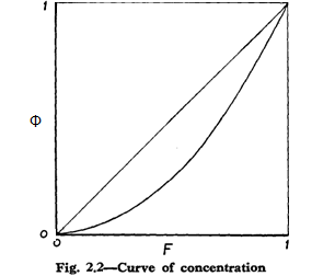
The curve of concentration must be convex to the F-axis, for we have
![]() ,
,
Which is positive since or origin is taken to the left of the start of the distribution. Also
![]() .
.
Thus the tangent to the curve makes a positive acute angle with the F-axis, and the angle increases as F increases; in other words, the curve is convex to the F-axis.
The area between the concentration curve and the line F = Φ is called the area of concentration. We proceed to show that it is equal to one-half the coefficient of concentration.
In fact, we have from Fig. 2.2
![]()
and thus
![]()
![]()
![]() .
.
Now
![]() ,
,
and hence
![]()
![]()
![]() .
.
Thus the area of
concentration is equal to ![]() , namely one-half of the coefficient of concentration
G at (2.29).
, namely one-half of the coefficient of concentration
G at (2.29).
2.26 Various methods have been given for calculating the mean difference. The following is probably the simplest, particularly for distributions specified in equal group-intervals.
Let us, without loss of generality, take an origin at the start of the distribution. We may then write
![]() ,
,
the summation Σ’ being taken over value such that j>k. We have also
![]() .
.
Thus
![]() ,
,
where Ch is the number of terms of type (x – xk) in Σ’ containing xh+1 – xh. Since h is the number of values of j less than or equal to h (the origin being at the start of the distribution) and N–h the number greater than or equal to h+1, we have Ch = h(N-h), and thus
![]()
![]()
This form is particularly useful if all the intervals are equal. Fh being the distribution function of xh we then have
![]()
![]() .
.
If the actual cumulated frequency for xh is Gh we have
![]() ,
,
the most convenient form in practice.
[End of Kendall and Stuart material.]
As mentioned above, the term Φ(x), which Kendall and Stuart refer to as the incomplete first moment, is often referred to, particularly in economics, as a Lorenz curve (after the person (Max O. Lorenz) who popularized its use (in 1905) for representing distribution of wealth). See the Wikipedia article http://en.wikipedia.org/wiki/Lorenz_curve for a description of the Lorenz curve. Using the notation of this article (replacing Φ by L), the Lorenz curve is given by
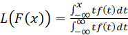 .
.
If the (cumulative) distribution function F(x) has a differentiable inverse, x(F), then the Lorenz curve is given by
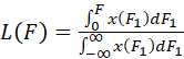 .
.
(If the inverse x(F) does not exist, the previous formula applies if x(F) is defined by x(F1) = inf{y|F(y)>F1}.)
The Wikipedia article on the Gini coefficient contains a number of formulas that maybe used to compute the value of the Gini coefficient from data. It also contains some interesting analytical formulas. Using the notation just introduced for the Lorenz curve (i.e., L(.)), the Gini coefficient is defined as:
![]() .
.
For a (cumulative) distribution function F(y) that is piecewise differentiable, has mean μ, and is zero for all negative values of y:
![]() .
.
Note that the assumption that the distribution function does not extend to minus infinity is essential here, since the integrals exist only if the distribution function starts at a finite value. For these formulas to apply, note that it is essential that the distribution function is zero for all negative values of y. (In general, similar formulas apply to any distribution function that starts (turns positive) at a finite value, in which case the lower limit of integration is that value. In economic applications the variate usually represents income or wealth, which are assumed to be positive.)
These formulas may be proved using integration by parts (see Wikipedia article posted at http://en.wikipedia.org/wiki/Integration_by_parts for information on integration by parts). The formula for integration by parts is
![]() .
.
We have
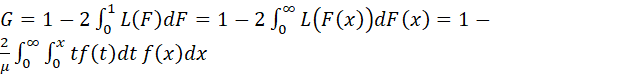 .
.
Let us apply integration by parts to the outer integral, using the functions
![]()
and
![]() .
.
Then the expression becomes (since the derivative of F(x) with respect to x is f(x))
![]() .
.
The second term on the right-hand side is equal to zero at both limits (it is here that the assumption that the distribution is zero for all negative values of x is used). Let us now apply integration by parts to the remaining term on the right-hand side, using the functions
![]()
and
![]() .
.
This yields
![]() .
.
The first term on the right-hand side is equal to zero at both limits, yielding the desired result:
![]() .
.
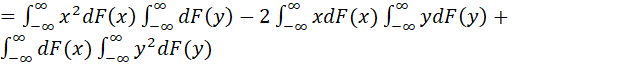
It now remains to prove that the second integral expression for G is equal to the first, i.e., that
![]() .
.
Multiplying through by μ, this is equivalent to proving
![]() .
.
The right-hand side reduces to
![]() .
.
Applying integration by parts with
![]()
and
![]()
yields
![]() .
.
The first term is equal to zero at both limits, and the second term is the definition of the mean, μ, which was to be proved.
Note that the assumption that the distribution starts at zero (or some other finite value) is essential in the above, because expressions such as
![]()
or
![]()
are undefined, whereas expressions such as
![]()
or
![]()
are well defined.
Recall Kendall and Stuart’s observation about the shortcoming of the Gini coefficient of concentration (and the Peason coefficient of variation):
“These coefficients both suffer from the disadvantage of being affected very much by μ1’, the value of the mean measured from some arbitrary origin, and are not usually employed unless there is a natural origin of measurement or comparisons are being made between distributions with similar origins.”
This observation is very appropriate. The value of the Gini coefficient is sensitive both to the choice of origin and to the value of the mean of the distribution. For distributions of income and wealth, the mean of the distribution is sensitive to the length of the right-hand “tail” of the distribution (i.e., to the skewness of the distribution). If the income or wealth of the richest portion of the population increases substantially relative to the income of the rest of the population, then the mean may shift considerably, and the value of the Gini coefficient may change substantially. That is, the values of a small portion of the population may have a substantial effect on the value of the Gini coefficient. This is basically what is happening in the United States today. A small number of people are becoming billionaires, while the income distribution of most of the population is not changing very much.
The shape of the Lorenz curve and the value of the Gini coefficient depend on the choice of origin for the Lorenz curve. In their discussion, Kendall and Stuart assume that the origin for F(x) and Φ(x) is taken at the starting point of the positive frequency. This results (plotting F(x) vs. Φ(x) as parametric functions of x) in Lorenz curves as depicted in the figure shown above, which start to rise from the point (0,0). If this origin is selected, then the Lorenz curve and the Gini coefficient are both invariant under scale and location transformations. In many applications, however, the Lorenz curve Φ(x) is plotted as a function of x, along with the distribution F(x). In this case, the Lorenz curve starts to rise at the point, x, at which the frequency (f(x)) becomes positive. In this case, the Gini coefficient is invariant with respect to scale transformations, but not with respect to location transformations. This point is not much appreciated, and will be discussed further, after considering some examples.
It is informative to examine values of the Gini coefficient (G) for a few different income (or wealth) distributions.
If all of the population has the same income, then the value of the Gini coefficient is zero (i.e., the line F=Φ is a straight line, so that the area between the curve of concentration and the diagonal line is zero).
If half of the population has no income and half has another income, the value of G is ½.
If the population consists of n individuals, and n-1 have half the income, equally shared, and one person has the other half, the value of G is ½.
The two preceding results may be seen graphically, by plotting the Lorenz curves, calculating the area between the diagonal line and the Lorenz curve, and doubling it. In the first case, the Lorenz curve goes from (0,0) to (0,.5) to (1,1), and in the second case the Lorenz curve goes from (0,0) to (1,.5) to (1,1). The areas of the two triangular areas are identical. This example is one illustration of how the income distribution may be very different in two instances, but the values of the Gini coefficients are the same.
If half the population has income a and half has income b>a, the value of G is (b-a)/(2(a+b)).
If the income is uniformly distributed over the interval 0 to some value, then the value of G is 1/3.
If the income is uniformly distributed over the interval from a to b>a, then the value of G is
![]() .
.
It is interesting to calculate this last result using the four different formulas for G given earlier i.e., the general formula involving the mean difference, the general formula involving the Lorenz curve, and the two special formulas when the distribution takes only non-negative values. First, using the general formula involving the mean difference, we have the following. Let x and y denote two independent selections from the uniform distribution over the interval from a to b. The density function for this distribution is 1/(b-a) for all values of the random variable in this interval, and zero elsewhere. We have:
![]()
![]()
![]()
![]()
![]()
![]()
![]()
![]()
![]() .
.
The mean of the distribution is μ=(a+b)/2. Hence
![]() .
.
Next, using the general formula, we have:
![]()
where
![]()
for x in the interval a to b and zero otherwise,
![]() ,
,
and
![]() .
.
Hence
![]() .
.
Since the random variable is positive, we may alternatively use the integral expressions to obtain this result. First, we have
![]()
for y in the interval between a and b and zero otherwise, so
![]() .
.
The first integral in the last term has value a. To evaluate the second integral in the last term, transform to z=(y-a)/(b-a), yielding
![]()
![]()
![]()
![]() .
.
Using the second integral formula for G, we have
![]()
![]() .
.
Transforming to z=(y-a)/(b-a), we have
![]()
![]()
![]() .
.
Using all four formulas we obtain, of course, the same result, G = (b-a)/((3(a+b)). In this particular example, the last formula was the easiest to use.
These examples show that, in general, some work is involved in calculating the value of the Gini coefficient. As observed by Kendall and Stuart, measures that involve absolute values, such as the mean difference, are generally more awkward to handle than those that do not, such as the variance. For random variables that are positive, the last formula is perhaps the simplest.
The above examples are not realistic examples of actual income distributions. In most countries, income distributions are skewed to the right, i.e., a few people earn most of the income (or possess most of the wealth). In these cases, the distribution of income appears similar to a log-normal distribution or to a Pareto distribution. For information about the Pareto distribution, see the Wikipedia article http://en.wikipedia.org/wiki/Pareto_distribution. The probability density function of a Pareto distribution is
![]()
for x>xm and 0 for x<xm. The distribution function is
![]()
for x>xm and 0 for x<xm. The mean, which is defined only if α>1, is αxm/(α-1). The median is
![]() .
.
The Lorenz curve for this Pareto distribution (defined only if α>1) is
![]()
and the Gini coefficient is
![]() .
.
Although the Gini coefficient is widely used to summarize income or wealth inequality, distributions that vary considerably can have the same value of the Gini coefficient. It is most useful for comparing two populations that are “similar” overall, such as the population of the United States in successive years. It is not very useful for comparing the income or wealth distributions of different countries – two countries may have similar values of the Gini coefficient for income (or wealth), but the shape of that distribution may differ substantially.
The Gini coefficient is used in a variety of applications to indicate the level of variability of the population. It is very sensitive to the value of the mean of the distribution, and has different values under translation (i.e., the value of G changes if the distribution is shifted, even if the shape is unchanged). For this reason, as observed by Kendall and Stuart, it is more appropriate when the origin of the distribution has some special natural significance. Since it is in general more complicated to calculate than the Pearson coefficient of variation (the standard deviation relative to the mean), it would appear that it has little to offer over that measure. Nevertheless, it is much used by economists and other social scientists as a general measure of inequality. Because it is so sensitive to the value of the mean, it would not appear to be a good choice in every situation. In cases in which particular aspects of a distribution are of interest, such as the “weight” or “length” of the upper tail of the distribution, much better measures would be quantile ratios, such as the ratio of total income earned by those in the top five percent of the income distribution, or the ratio of the mean income for the highest five-percent quantile to the mean income of the lower 95-percent quantile.
FndID(128)
FndTitle(Miscellany 55: The Widening Income Distribution in the United States)
FndDescription(Miscellany 55: The Widening Income Distribution in the United States)
FndKeywords(income distritution; gini coefficient; widening income distribution)